Text Analytics in Python

El curso a partir del cual está basada esta pagina se refería a Natural language processing, no Text Analytics. Sin embargo creo que se tratan aspectos que no son sólo de Natural language processing.

https://en.wikipedia.org/wiki/Natural_language_processing

Natural language processing (NLP) is concerned with the interactions between computers and human (natural) languages, in particular how to process and analyze large amounts of natural language data.

Challenges in Natural Language Processing frequently involve text classification, speech recognition, natural language understanding, and natural language generation.

Natural Language Processing basically consists of combining machine learning techniques with text, and using math and statistics to get that text in a format that the machine learning algorithms can understand.

Some Resources

NLTK

https://www.nltk.org/

Online book: http://www.nltk.org/book/

https://en.wikipedia.org/wiki/Natural_Language_Toolkit

The Natural Language Toolkit, or more commonly NLTK, is a suite of libraries and programs for symbolic and statistical natural language processing (NLP) for English written in the Python programming language.

Installation

http://www.nltk.org/install.html

conda install nltk  # Installs nltk

Installing NLTK Data

https://www.nltk.org/data.html

NLTK comes with many corpora, toy grammars, trained models, etc. A complete list is posted at: http://nltk.org/nltk_data/

import nltk         # Imports the library
nltk.download()     # Download the necessary datasets

I have installed it using Jupyter-notebook. I install the data in this location: /home/adelo/.nltk/nltk_data

You will need to set the NLTK_DATA environment variable to specify the location of the data: /home/adelo/.bashrc

# Installing NLTK Data
export NLTK_DATA=/home/adelo/.nltk/nltk_data

Test that the data has been installed as follows (This assumes you downloaded the Brown Corpus):

from nltk.corpus import brown
brown.words() 
# Output:
['The', 'Fulton', 'County', 'Grand', 'Jury', 'said', ...]

First example

Our test dataset

We'll be using the SMS Spam Collection DataSet. This dataset can be downloaded from https://archive.ics.uci.edu/ml/datasets/SMS+Spam+Collection#

Text file: smsspamcollection

The SMS Spam Collection v.1 (hereafter the corpus) is a set of SMS tagged messages that have been collected for SMS Spam research. It contains one set of SMS messages in English of 5,574 messages, tagged acording being ham (legitimate) or spam.

The SMS Spam Collection v.1 has a total of 4,827 SMS legitimate messages (86.6%) and a total of 747 (13.4%) spam messages.

The files contain one message per line. Each line is composed by two columns: one with label (ham or spam) and other with the raw text. Here are some examples:

ham   What you doing?how are you?
ham   Ok lar... Joking wif u oni...
ham   dun say so early hor... U c already then say...
ham   MY NO. IN LUTON 0125698789 RING ME IF UR AROUND! H*
ham   Siva is in hostel aha:-.
ham   Cos i was out shopping wif darren jus now n i called him 2 ask wat present he wan lor. Then he started guessing who i was wif n he finally guessed darren lor.
spam   FreeMsg: Txt: CALL to No: 86888 & claim your reward of 3 hours talk time to use from your phone now! ubscribe6GBP/ mnth inc 3hrs 16 stop?txtStop
spam   Sunshine Quiz! Win a super Sony DVD recorder if you canname the capital of Australia? Text MQUIZ to 82277. B
spam   URGENT! Your Mobile No 07808726822 was awarded a L2,000 Bonus Caller Prize on 02/09/03! This is our 2nd attempt to contact YOU! Call 0871-872-9758 BOX95QU

Note: messages are not chronologically sorted.

Using these labeled ham and spam examples, we'll train a machine learning model to learn to discriminate between ham/spam automatically. Then, with a trained model, we'll be able to classify arbitrary unlabeled messages as ham or spam.

Importing the data

messages = [line.rstrip() for line in open('smsspamcollection/SMSSpamCollection')]
print(len(messages))

# Output:
5574

Let's print the first ten messages and number them using enumerate:

for message_no, message in enumerate(messages[:10]):
    print(message_no, message)
    print('\n')

# Output:
0 ham	Go until jurong point, crazy.. Available only in bugis n great world la e buffet... Cine there got amore wat...


1 ham	Ok lar... Joking wif u oni...


2 spam	Free entry in 2 a wkly comp to win FA Cup final tkts 21st May 2005. Text FA to 87121 to receive entry question(std txt rate)T&C's apply 08452810075over18's


3 ham	U dun say so early hor... U c already then say...


4 ham	Nah I don't think he goes to usf, he lives around here though


5 spam	FreeMsg Hey there darling it's been 3 week's now and no word back! I'd like some fun you up for it still? Tb ok! XxX std chgs to send, £1.50 to rcv


6 ham	Even my brother is not like to speak with me. They treat me like aids patent.


7 ham	As per your request 'Melle Melle (Oru Minnaminunginte Nurungu Vettam)' has been set as your callertune for all Callers. Press *9 to copy your friends Callertune


8 spam	WINNER!! As a valued network customer you have been selected to receivea £900 prize reward! To claim call 09061701461. Claim code KL341. Valid 12 hours only.


9 spam	Had your mobile 11 months or more? U R entitled to Update to the latest colour mobiles with camera for Free! Call The Mobile Update Co FREE on 08002986030

Due to the spacing we can tell that this is a TSV ("tab separated values") file, where the first column is a label saying whether the given message is a normal message (commonly known as "ham") or "spam". The second column is the message itself. (Note our numbers aren't part of the file, they are just from the enumerate call).

Instead of parsing TSV manually using Python, we can just take advantage of pandas! Let's go ahead and import it into a DataFrame:

import pandas as pd

messages = pd.read_csv('smsspamcollection/SMSSpamCollection', sep='\t',
                           names=["label", "message"])

type(messages)
# Output:
pandas.core.frame.DataFrame

messages.head()
# output:
    label                                              message
0     ham     Go until jurong point, crazy.. Available only ...
1     ham                         Ok lar... Joking wif u oni...
2    spam     Free entry in 2 a wkly comp to win FA Cup fina...
3     ham     U dun say so early hor... U c already then say...
4     ham     Nah I don't think he goes to usf, he lives aro...

Exploratory Data Analysis

	Method / Operator / Description	Example
Describe the data	`import pandas` `df.describe()`	import pandas messages.describe() # Output: label message count 5572 5572 unique 2 5169 top ham Sorry, I'll call later freq 4825 30
Describe by group	`import pandas` `df.groupby('label').describe()` Let's use groupby to use describe by label. This way we can begin to think about the features that separate ham and spam!	import pandas messages.groupby('label').describe() # Output: message label ham count 4825 unique 4516 top Sorry, I'll call later freq 30 spam count 747 unique 653 top Please call our customer service representativ... freq 4
Text length	`df['length'] = df['colums'].apply(len)` Let's make a new column to detect how long the text messages are.	messages['length'] = messages['message'].apply(len) messages.head() # Output: label message length 0 ham Go until jurong point, crazy.. Available only ... 111 1 ham Ok lar... Joking wif u oni... 29 2 spam Free entry in 2 a wkly comp to win FA Cup fina... 155 3 ham U dun say so early hor... U c already then say... 49 4 ham Nah I don't think he goes to usf, he lives aro... 61
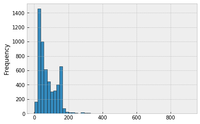
Histogram	Play around with the bin size! From the `Histogram`, it looks like text length may be a good feature to think about! Let's try to explain why the x-axis of the Histogram goes all the way to 1000ish. This must mean that there is some really long message!	import matplotlib.pyplot as plt import seaborn as sns %matplotlib inline plt.style.use('bmh') messages['length'].plot(bins=50, kind='hist', edgecolor="k")
	Using `describe()` over the `length we can see` that there is a message of 910 characters. This is why the x-axis of the Histogram above goes all the way to 1000ish. Let's use masking to find this message.	messages.length.describe() # Output: count 5572.000000 mean 80.489950 std 59.942907 min 2.000000 25% 36.000000 50% 62.000000 75% 122.000000 max 910.000000
	This way we can find the message of 910 characters.	messages[messages['length'] == 910]['message'].iloc[0] # Output: "For me the love should start with attraction.i should feel that I need her every time around me.she should be the first thing which comes in my thoughts.I would start the day and end it with her.she should be there every time I dream.love will be then when my every breath has her name.my life should happen around her.my life will be named to her.I would cry for her.will give all my happiness and take all her sorrows.I will be ready to fight with anyone for her.I will be in love when I will be doing the craziest things for her.love will be when I don't have to proove anyone that my girl is the most beautiful lady on the whole planet.I will always be singing praises for her.love will be when I start up making chicken curry and end up makiing sambar.life will be the most beautiful then.will get every morning and thank god for the day because she is with me.I would like to say a lot..will tell later.."
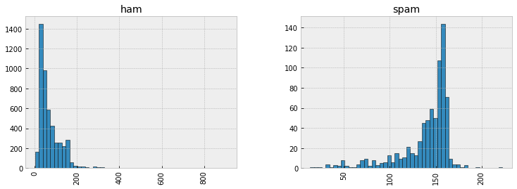
	Let's focus back on the idea of trying to see if message length is a distinguishing feature between ham and spam. Very interesting! Through just basic EDA we've been able to discover a trend that spam messages tend to have more characters.	messages.hist(column='length', by='label', bins=50,figsize=(12,4), edgecolor="k")

Text Pre-processing

Our main issue with our data is that it is all in text format (strings). The classification algorithms that we've learned about so far will need some sort of numerical feature vector in order to perform the classification task. There are actually many methods to convert a corpus to a vector format. The simplest is the the bag-of-words approach, where each unique word in a text will be represented by one number.

In this section we'll convert the raw messages (sequence of characters) into vectors (sequences of numbers).

As a first step, let's write a function that will split a message into its individual words and return a list. We'll also remove very common words, ('the', 'a', etc..). To do this we will take advantage of the NLTK library. It's pretty much the standard library in Python for processing text and has a lot of useful features. We'll only use some of the basic ones here.

Let's create a function that will process the string in the message column, then we can just use apply() in pandas do process all the text in the DataFrame.

First removing punctuation. We can just take advantage of Python's built-in string library to get a quick list of all the possible punctuation.

		Example
Removing punctuation	We can just take advantage of Python's built-in string library to get a quick list of all the possible punctuation: `string.punctuation`	import string mess = 'Sample message! Notice: it has punctuation.' # Check characters to see if they are in punctuation nopunc = [char for char in mess if char not in string.punctuation] # Join the characters again to form the string. nopunc = ''.join(nopunc) print(nopunc) # Output: Sample message Notice it has punctuation
Remove stopwords	Stopwords are very common words ('the', 'a', etc..). We can import a list of english stopwords from NLTK (check the documentation for more languages and info).	from nltk.corpus import stopwords stopwords.words('english')[0:10] # Show some stop words # Output: ['i', 'me', 'my', 'myself', 'we', 'our', 'ours', 'ourselves', 'you', 'your'] nopunc.split() # Output: ['Sample', 'message', 'Notice', 'it', 'has', 'punctuation'] # Now just remove any stopwords clean_mess = [word for word in nopunc.split() if word.lower() not in stopwords.words('english')] clean_mess # Output: ['Sample', 'message', 'Notice', 'punctuation']
Making a function to apply a set of pre-procesteps steps and tokarize the data `Remove Punctuation` `Remove Stopwords` `Tokenize`	We can make a function to to remove `Punctuation`, `Stopwords` and `Tokenize` our messages. This function will be applied to our DataFrame. `Tokenization` is just the term used to describe the process of converting the normal text strings in to a list of tokens (words that we actually want). Notice that this function is returning a `list` of words without Punctuation or Stopwords.	def text_process(mess): """ Takes in a string of text, then performs the following: 1. Remove all punctuation 2. Remove all stopwords 3. Returns a list of the cleaned text """ # Check characters to see if they are in punctuation nopunc = [char for char in mess if char not in string.punctuation] # Join the characters again to form the string. nopunc = ''.join(nopunc) # Now just remove any stopwords return [word for word in nopunc.split() if word.lower() not in stopwords.words('english')]
Applying the function over our DataFrace	Note: We may get some warnings or errors for symbols we didn't account for or that weren't in Unicode (like a British pound symbol)	# Show original dataframe messages.head() # Output: label message length 0 ham Go until jurong point, crazy.. Available only ... 111 1 ham Ok lar... Joking wif u oni... 29 2 spam Free entry in 2 a wkly comp to win FA Cup fina... 155 3 ham U dun say so early hor... U c already then say... 49 4 ham Nah I don't think he goes to usf, he lives aro... 61 # Applying the function messages['message'].head(5).apply(text_process) # Output 0 [Go, jurong, point, crazy, Available, bugis, n... 1 [Ok, lar, Joking, wif, u, oni] 2 [Free, entry, 2, wkly, comp, win, FA, Cup, fin... 3 [U, dun, say, early, hor, U, c, already, say] 4 [Nah, dont, think, goes, usf, lives, around, t...
Continuing Normalization	There are a lot of ways to continue normalizing this text. Such as `Stemming` or `distinguishing by part of speech`. NLTK has lots of built-in tools and great documentation on a lot of these methods. Sometimes they don't work well for text-messages due to the way a lot of people tend to use abbreviations or shorthand, For example: `'Nah dawg, IDK! Wut time u headin to da club?'` Vs. `'No dog, I don't know! What time are you heading to the club?'`

Vectorization

Usually, after pre-processing, we have the messages as lists of tokens (also known as lemmas).

Now we'll convert each message, represented as a list of tokens (lemmas) into a Numeric Vector that machine learning models can understand.

To be able to run a Machine Learning algorithm, we first need to transform each text document into a numerical representation in the form of a vector. This matrix will be the numerical representation that a Machine Learning algorithm is able to understand.

We'll do that in three steps using the bag-of-words model:

Create the Document Term Matrix (DTM) (Also know as Term Frequency(TF)): Count how many times does a word occur in each text document.
Term weighting: Weigh the counts, so that frequent tokens get lower weight (Inverse Document Frequency).
Normalization: Normalize the vectors to unit length, to abstract from the original text length (L2 Norm).

Document Term Matrix

We will convert a collection of text documents to a matrix of token counts:

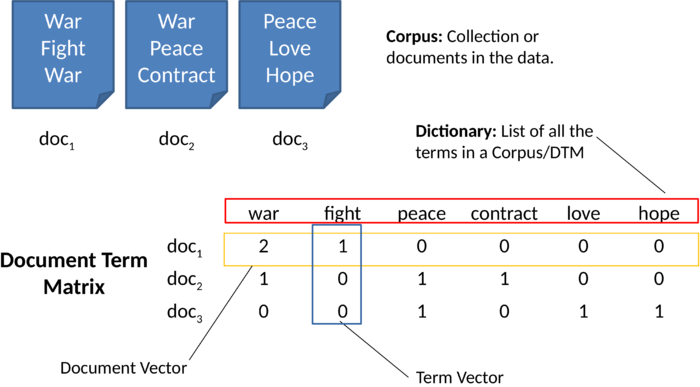
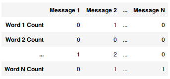
We can imagine a matrix of token counts as a 2-Dimensional matrix. Where the 1-dimension is the entire vocabulary (1 row per word) and the other dimension are the actual documents, in this case a column per text message.

Since there are so many messages, we can expect a lot of zero counts for the presence of that word in that document. Because of this, SciKit-Learn will output a Sparse Matrix.

Each columns (or row depending on the approach) of this matrix represent a word in the training data. Thus, each document is defined by the frequency of the words that are in the dictionary composed for all the terms in our data.


Figure 1: The Document-Term Matrix File:Document-Term Matrix.pdf File:Document-Term Matrix.ods File:Using text mining and Machine Learning to classify documents.pdf

Using Scikit-learn CountVectorizer method to create a DTM

In Python, we can use Scikit-learn's CountVectorizer method to create a DTM. Let's see how to do so in our example:

from sklearn.feature_extraction.text import CountVectorizer


# This create a «Bag-of-Words (bow) transformed object» (It is not the resulting DTM yet)
# There are a lot of arguments and parameters that can be passed to the CountVectorizer. In this case we will just specify the analyzer to be our own previously defined function «text_process»:
# Might take a while...
bow_transformer = CountVectorizer(analyzer=text_process).fit(messages['message'])


# Print total number of vocab words:
print(len(bow_transformer.vocabulary_))
# Output:
11425


# Let's take one text message and get its bag-of-words counts as a vector, putting to use our new bow_transformer:
message4 = messages['message'][3]
print(message4)
# Output:
U dun say so early hor... U c already then say...


# Now let's see its vector representation:
bow4 = bow_transformer.transform([message4])
print(bow4)
print(bow4.shape)
# Output:
(0, 4068)   2
(0, 4629)   1
(0, 5261)   1
(0, 6204)   1
(0, 6222)   1
(0, 7186)   1
(0, 9554)   2
(1, 11425)
# This means that there are seven unique words in message number 4 (after removing common stop words). Two of them appear twice, the rest only once.


# Let's go ahead and check and confirm which ones appear twice:
print(bow_transformer.get_feature_names()[4068])
print(bow_transformer.get_feature_names()[9554])
# Output:
U
say


# Now we can use «.transform» on our «Bag-of-Words (bow) transformed object» and transform the entire DataFrame of messages. Let's go ahead and check out how the bag-of-words counts for the entire SMS corpus is a large, sparse matrix:
messages_bow = bow_transformer.transform(messages['message'])


print('Shape of Sparse Matrix: ', messages_bow.shape)
print('Amount of Non-Zero occurences: ', messages_bow.nnz)
# Output:
Shape of Sparse Matrix:  (5572, 11444)
Amount of Non-Zero occurences:  50795


sparsity = (100.0 * messages_bow.nnz / (messages_bow.shape[0] * messages_bow.shape[1]))
print('sparsity: {}'.format(round(sparsity)))
# Output:
sparsity: 0

Term weighting and Normalization using TF-IDF

In general terms, the process of weighting involves emphasizing the contribution of particular aspects of a phenomenon (or of a set of data) over others to a final outcome or result; thereby highlighting those aspects in comparison to others in the analysis. That is, rather than each variable in the data set contributing equally to the final result, some of the data is adjusted to make a greater contribution than others. https://en.wikipedia.org/wiki/Weighting

TF-IDF, short for Term Frequency–Inverse Document Frequency, and the TF-IDF Weight, is a statistical measure used to evaluate how important a word is to a document in a collection or corpus. It has many uses, most importantly in automated text analysis. It is often used as a weighting factor in machine learning algorithms for Natural Language Processing.

Typically, the TF-IDF Weight is computed by the product of the TF and the IDF

The normalized Term Frequency (TF), which is the number of times a word appears in a document, divided by the total number of words in that document.
Why Normalization?: Since every document is different in length, it is probably that a term would appear much more times in long documents than shorter ones. Thus, the Term Frequency is often divided by the document length (total number of words in that document) as a way of Normalization:

$TF(t)={\frac {{\text{Number of times term }}t{\text{ appears in a document}}}{\text{Total number of terms in that document}}}$

Inverse Document Frequency (IDF). The IDF measures how important a term is. While computing TF, all terms are considered equally important. However it is known that certain terms, such as "is", "of", and "that", may appear a lot of times but have little importance. Thus we need to weigh down the frequent terms while scale up the rare ones, by computing the following:
The IDF is computed as the logarithm of the number of the documents in the corpus divided by the number of documents where the specific term appears.

$IDF(t)=\ln {\Bigl (}{\frac {\text{Total number of documents}}{{\text{Number of documents with term }}t{\text{ in it}}}}{\Bigr )}$

$IF{\text{-}}IDF(t)=TF(t)*IDF(t)$

Example:

Consider a document containing 100 words wherein the word cat appears 3 times.

Then, the normalized Term Frequency for cat is:

$TF(cat)={\frac {3}{100}}=0.03$

Now, assume we have 10 million documents and the word cat appears in one thousand of these.

Then, the Inverse Document Frequency for cat is:

$IDF(cat)=\ln {\Bigl (}{\frac {10000000}{1000}}{\Bigr )}=4$

Finally, the TF-IDF Weight is the product of these quantities:

$IF{\text{-}}IDF(cat)=TF(cat)*IDF(cat)=0.03*4=0.12$

Using TfidfTransformer method from Scikit-learn to compute the TF-IDF

Term weighting and Normalization can be done with TF-IDF, using scikit-learn's TfidfTransformer.

from sklearn.feature_extraction.text import TfidfTransformer

tfidf_transformer = TfidfTransformer().fit(messages_bow)
tfidf4 = tfidf_transformer.transform(bow4)
print(tfidf4)
# Output:
(0, 9554)     0.5385626262927564
(0, 7186)     0.4389365653379857
(0, 6222)     0.3187216892949149
(0, 6204)     0.29953799723697416
(0, 5261)     0.29729957405868723
(0, 4629)     0.26619801906087187
(0, 4068)     0.40832589933384067

We'll go ahead and check what is the IDF (inverse document frequency) of the word "u" and of word "university"?

print(tfidf_transformer.idf_[bow_transformer.vocabulary_['u']])
print(tfidf_transformer.idf_[bow_transformer.vocabulary_['university']])
# Output:
3.28005242674
8.5270764989

To transform the entire bag-of-words corpus into TF-IDF corpus at once:

messages_tfidf = tfidf_transformer.transform(messages_bow)
print(messages_tfidf.shape)
# Output:
(5572, 11425)

Training the model

With messages represented as vectors, we can finally train our spam/ham classifier. Now we can actually use almost any sort of classification algorithms. For a variety of reasons, the Naive Bayes classifier algorithm is a good choice.

Naive Bayes classifier using scikit-learn

from sklearn.naive_bayes import MultinomialNB
spam_detect_model = MultinomialNB().fit(messages_tfidf, messages['label'])

Let's try classifying our single random message and checking how we do:

print('predicted:', spam_detect_model.predict(tfidf4)[0])
print('expected:', messages.label[3])
# Output:
predicted: ham
expected: ham

Model Evaluation

all_predictions = spam_detect_model.predict(messages_tfidf)
print(type(all_predictions))
print(len(all_predictions))
print(all_predictions)

# Output:
<class 'numpy.ndarray'>
5572
['ham' 'ham' 'spam' ... 'ham' 'ham' 'ham']

We can use SciKit-Learn's built-in classification report, which returns precision, recall, f1-score, and a column for support (meaning how many cases supported that classification). Check out the links for more detailed info on each of these metrics and the figure below:

Precision and recall

from sklearn.metrics import classification_report
print (classification_report(messages['label'], all_predictions))

# Output:
               precision    recall  f1-score   support

        ham         0.98      1.00      0.99      4825
       spam         1.00      0.85      0.92       747

avg / total         0.98      0.98      0.98      5572

There are quite a few possible metrics for evaluating model performance. Which one is the most important depends on the task and the business effects of decisions based off of the model. For example, the cost of mis-predicting "spam" as "ham" is probably much lower than mis-predicting "ham" as "spam".

In the above "evaluation", we evaluated accuracy on the same data we used for training. You should never actually evaluate on the same dataset you train on!

A proper way is to split the data into a training/test set, where the model only ever sees the training data during its model fitting and parameter tuning. The test data is never used in any way. This is then our final evaluation on test data is representative of true predictive performance.

Train Test Split

from sklearn.model_selection import train_test_split

msg_train, msg_test, label_train, label_test = \
train_test_split(messages['message'], messages['label'], test_size=0.2)

print(len(msg_train), len(msg_test), len(msg_train) + len(msg_test))

# Output
4457 1115 5572

The test size is 20% of the entire dataset (1115 messages out of total 5572), and the training is the rest (4457 out of 5572). Note the default split would have been 30/70.

Creating a Data Pipeline

Let's run our model again and then predict off the test set. We will use SciKit Learn's pipeline capabilities to store a pipeline of workflow. This will allow us to set up all the transformations that we will do to the data for future use. Let's see an example of how it works:

from sklearn.pipeline import Pipeline

pipeline = Pipeline([
    ('bow', CountVectorizer(analyzer=text_process)),  # strings to token integer counts
    ('tfidf', TfidfTransformer()),  # integer counts to weighted TF-IDF scores
    ('classifier', MultinomialNB()),  # train on TF-IDF vectors w/ Naive Bayes classifier
])

Now we can directly pass message text data and the pipeline will do our pre-processing for us! We can treat it as a model/estimator API:

pipeline.fit(msg_train,label_train)

# Output:
Pipeline(steps=[('bow', CountVectorizer(analyzer=<function text_process at 0x11e795bf8>, binary=False,
        decode_error='strict', dtype=<class 'numpy.int64'>,
        encoding='utf-8', input='content', lowercase=True, max_df=1.0,
        max_features=None, min_df=1, ngram_range=(1, 1), preprocessor=None,...f=False, use_idf=True)), ('classifier', MultinomialNB(alpha=1.0, class_prior=None, fit_prior=True))])

predictions = pipeline.predict(msg_test)

print(classification_report(predictions,label_test))

# Output:
                precision    recall  f1-score   support

        ham          1.00      0.96      0.98      1001
       spam          0.75      1.00      0.85       114

avg / total          0.97      0.97      0.97      1115

Now we have a classification report for our model on a true testing set!

There is a lot more to Natural Language Processing than what we've covered here, and its vast expanse of topics could fill up several college courses!