Big Data Integration

File:Exploration of the Darts dataset using statistics.pdf

Big data introduction

What Is Big Data?: Big Data is such a huge and complex data that cannot be stored or processed easily using traditional data processing techniques/tools.

Unstructured data comes from information that is not organized or easily interpreted by traditional databases or data models, and typically, it’s text-heavy. Metadata, Twitter tweets, and other social media posts are good examples of unstructured data.

Multi-structured data refers to a variety of data formats and types and can be derived from interactions between people and machines, such as web applications or social networks. A great example is web log data, which includes a combination of text and visual images along

Scaling a database

• Typical problems encountered when scaling a traditional database:

• More than 30,000 gigabytes of data are generated every second.

• The data is diverse nowadays

• Traditional database systems, such as relational databases, have been pushed to the limit.
• A new breed of technologies has emerged under the term NoSQL.

• These systems can scale to vastly larger sets of data.

• Applications using normalized database schema require the use of join's, which doesn't perform well under lots of data and/or nodes.
• Existing RDBMS clustering solutions require scale-up, which is limited & not really scalable when dealing with exponential growth.
• Machines have upper limits on capacity, & sharding the data & processing across machines is very complex & app-specific.

• Scaling with a Queue:

• Timeout error on inserting to the database. The database can't keep up with the load, so write requests are timing out.
• Instead of having the web server hit the database directly, you insert a queue between the web server and the database.
• If the database ever gets overloaded again, the queue will just get bigger instead of timing out to the web server and potentially losing data.
• Unfortunately, if the growing continues, adding a queue and doing batch updates was only a band-aid for the scaling problem.

• Scaling by Sharding the Database:

• Sharding is a type of database partitioning that separates very large databases into smaller, faster, more easily managed parts called data shards.
• To use multiple database servers and spread the table across all the servers. Each server will have a subset of the data for the table.
• You have to modify your top-100-URLs query to get the top 100 URLs from each shard and merge those together for the global top 100 URLs.
• As the application gets more and more popular, you keep having to reshard the database into more shards to keep up with the write load.
• Eventually you have so many shards that it becomes a challenge to manage all requests in a single transaction in case of any error or problems.

• As the simple web analytics application evolved, the system continued to get more and more complex: queues, shards, replicas, resharding scripts, and so on.
• One problem is that your database is not self-aware of its distributed nature, so it can’t help you to deal with shards, replication, and distributed queries. All that complexity got pushed to you both in operating the database and developing the application code.
• The system is not engineered for human mistakes. Quite the opposite, the system keeps getting more and more complex, making it more and more likely that a mistake will be made.
• Human-fault tolerance is not optional. It’s essential, especially when Big Data adds so many more complexities to building applications.

• How will Big Data Techniques help?:

• Databases and computation systems used for Big Data are aware of their distributed nature. So things like sharding and replication are handled for you.
• When it comes to scaling, you’ll just add nodes, and the systems will automatically rebalance onto the new nodes.
• Immutable data: when you make a mistake, you might write bad data, but at least you won’t destroy good data. This is a much stronger human-fault tolerance guarantee than in a traditional system based on mutation.
• With traditional databases, you’d be wary of using immutable data because of how fast such a dataset would grow. But because Big Data techniques can scale to so much data, you have the ability to design systems in different ways.
• Immutable - unchanging over time or unable to be changed.

NoSQL

A NoSQL (originally referring to "non SQL" or "non relational") database provides a mechanism for the storage and retrieval of data which is modelled other than the tabular relations used in the relational databases.

• Such databases have existed since the late 1960s, but did not obtain the name as "NoSQL".
• Facebook, Google and eBay initiated the need and usage of NoSQL databases in big data and real-time web applications.
• NoSQL systems are also called “Not only SQL” to emphasize that they may support SQL-like query languages.

• NoSQL is for situations when the user is unsure of what structure to use for the data.
• One common physical structure used by NoSQL is a string of key-value pairs.
• A NoSQL technology adds a special application programming interface (API) to SQL to allow SQL to work with data not stored in the traditional relational table format.
• NoSQL has the ability to handle large volumes of unstructured data faster and more efficiently than traditional relational database management systems.

Why NoSQL is not a panacea

• Hadoop and databases such as Cassandra and Riak systems can handle very large amounts of data, but with serious trade-offs.

• Hadoop, for example, can parallelize large-scale batch computations on very large amounts of data, but the computations have high latency. You don’t use Hadoop for anything where you need low-latency results.

• NoSQL databases like Cassandra achieve their scalability by offering you a much more limited data model than you’re used to with something like SQL. Squeezing your application into these limited data models can be very complex.

• These tools on their own are not a panacea. But when intelligently used in conjunction with one another, you can produce scalable systems for arbitrary data problems with human-fault tolerance and a minimum of complexity.

Service-Oriented Architecture (SOA)

• A service-oriented architecture (SOA) is a style of software design where services are provided to the other components by application components, through a communication protocol over a network.

• A service is a discrete unit of functionality that can be accessed remotely and acted upon and updated independently, such as retrieving a credit card statement online.

• SOA provides access to reusable Web services over a TCP/IP network,

Web services

• A software component stored on one computer that can be accessed via method calls by an application (or other software component) on another computer over a network

• Web services communicate using such technologies as:
  • XML, JSON and HTTP
  • Simple Object Access Protocol (SOAP): An XML-based protocol that allows web services and clients to communicate in a platform-independent manner

Why Web services:

• By using web services, companies can spend less time developing new applications and can create new applications in an innovative way in small amount of time.
• Amazon, Google, eBay, PayPal and many others make their server-side applications available to their partners via web services.

Basic concepts:

• Remote machine or server: The computer on which a web service resides
• A client application that accesses a web service sends a method call over a network to the remote machine, which processes the call and returns a response over the network to the application
• Publishing (deploying) a web service: Making a web service available to receive client requests.
• Consuming a web service: Using a web service from a client application.
• In Java, a web service is implemented as a class that resides on a server.

An application that consumes a web service (client) needs:

• An object of a proxy class for interacting with the web service.
• The proxy object handles the details of communicating with the web service on the client's behalf

JAX-WS:

• The Java API for XML Web Services (JAX-WS) is a Java programming language API for creating web services, particularly SOAP services. JAX-WS is one of the Java XML programming APIs. It is part of the Java EE platform.
  • Requests to and responses from web services are typically transmitted via SOAP.
  • Any client capable of generating and processing SOAP messages can interact with a web service, regardless of the language in which the web service is written.

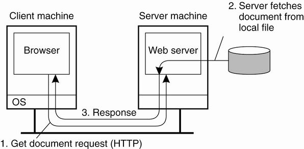
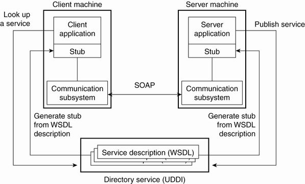
Traditional Web-Based Systems vs Web Services-Based Systems:

Traditional Web-Based Systems

Web services based systems

Creating - Deploying and Testing a Java Web Service using NetBeans

Esta sección fue realizada a partir de la siguiente presentación, la cual forma parte del material del curso de Big Data del Prof. Muhammad Iqbal: File:Lecture_4-Big_Data_integration-Web_Service.pptx

El proyecto NetBeans que contiene el Java Web Service resultante de este tutorial: File:CalculatorWSApplication.zip

Netbeans 6.5 - 9 and Java EE enable programmers to "publish (deploy)" and/or "consume (client request)" web services In Netbeans, you focus on the logic of the web service and let the IDE handle the web service's infrastructure.

• We first need to to do some configuration in NetBeans:
  • Go to /usr/local/netbeans-8.2/etc/netbeans.conf:
    • Find the line: netbeans_default_options
    • If -J-Djavax.xml.accessExternalSchema=all is not between the quotes then paste it in.

• If you are deploying to the GlassFish Server you need to modify the configuration file of the GlassFish Server (domain.xml):
  • /usr/local/glassfish-4.1.1/glassfish/domains/domain1/config/domain.xml
    • Find : <java-config
    • Check the jvm-options for the following configuration: <jvm-options>-Djavax.xml.accessExternalSchema=all</jvm-options>
    • It should be there by default, if not paste it in, save file and exit
    • You can now start Netbeans IDE

• Create a Web Service in NetBeans- Locally
  • Choose File > New Project:
  • Select Web Application from the Java Web category
  • Change Project Name: to CalculatorWSApplication
  • Set the server to GlassFish 4.1.1
  • Set Java EE Version: Java EE 7 Web
  • Set Context path: /CalculatorWSApplication
  • After that you should now have a project created in the Projects view on the left hand side.

• Creating a WS from a Java Class:

• Right-click the CalculatorWSApplication node and choose New > Web Service.

• If the option is not there choose Other > Web Services > Web Service

• Click Next
• Name the web service CalculatorWS and type com.hduser.calculator in Package. Leave Create Web Service from Scratch selected.
• Select Implement Web Service as a Stateless Session Bean.
• Click Finish. The Projects window displays the structure of the new web service and the Java class (CalculatorWS.java) is generate and automatically shown in the editor area. A default hello web service is created by Netbeans.

• Adding an Operation to the WS (CalculatorWS.java):

• Open CalculatorWS.java WS.
• Change to the Design view in the editor.
• Click the Add operation button.
• In the upper part of the Add Operation dialog box, type add in Name and type int' in the Return Type drop-down list.
• In the lower part of the Add Operation dialog box, click Add and create a parameter of type int named num_1.
• Click Add again and create a parameter of type int called num_2.
• Click OK at the bottom of the panel to add the operation.
• Remove the default hello operation: Right click on hello operation and choose: Remove Operation
• Click on the source view to go back to view the code in the editor.
• You will see the default hello code is gone and the new add method is now there instead.
• Now we have to alter the code to look like this.

package com.adelo.calculator;

import javax.jws.WebService;
import javax.jws.WebMethod;
import javax.jws.WebParam;
import javax.ejb.Stateless;

@WebService(serviceName = "CalculatorWS")
@Stateless()
public class CalculatorWS {

    /**
     * Web service operation
     */
    @WebMethod(operationName = "add")
    public int add(@WebParam(name = "num_1") int num_1, @WebParam(name = "num_2") int num_2) {
        //TODO write your implementation code here:
        int result = num_1 + num_2;
        return result;
    }
}

• Well done, you have just created your first Web Service.

• To test the Web service drop down the Web Services directory and right click on CalculatorWSApplication.
• Choose Test Web service.
• Netbeans throws an error: It is letting us know that we have not deployed our Web Service.

• Right click on the main Project node and select deploy

• Testing the WS:

• Deploying the Web Service will automatically start the GlassFish server. Allow the server to start, this will take a little while. You can check the progress by clicking on the GlassFish tab at the bottom of the IDE.
• Wait until you see: «CalculatorWSApplication was successfully deployed in 9,912 milliseconds»
• Now you can right click on the Web Service as before and choose Test Web Service.
• The browser will open and you can now test the Web service and view the WSDL file.
• You can also view the Soap Request and Response.

Understanding a Web Service Java Class

• Each new web service class created with the JAX-WS APIs is a POJO (plain old Java object)

• You do not need to extend a class or implement an interface to create a Web service.

• When you compile a class that uses the following JAX-WS 2.0 annotations, the compiler creates the compiled code framework that allows the web service to wait for and respond to client requests:

• @WebService(«Optional elements»)

• Indicates that a class represents a web service.
• Optional element name specifies the name of the proxy class that will be generated for the client.
• Optional element serviceName specifies the name of the class that the client uses to obtain a proxy object.
• Netbeans places the @WebService annotation at the beginning of each new web service class you create.
• You can add the optional name and serviceName this way: @WebService(serviceName = "CalculatorWS")

• @WebMethod(«Optional elements»)

• Methods that are tagged with the @WebMethod annotation can be called remotely.
• Methods that are not tagged with @WebMethod are not accessible to clients that consume the web service.
• Optional operationName element to specify the method name that is exposed to the web service's client.

• @WebParam annotation(«Optional elements»)

• Optional element name indicates the parameter name that is exposed to the web service's clients.

Consuming the Web Service

Netbeans 6.5 - 9 and Java EE enable programmers to "publish (deploy)" and/or "consume (client request)" web services

Creating a Java Web Application that consumes a Web Service

El proyecto NetBeans resultante de esta sección: File:CalculatorWSJSPClient.zip

• Now that we have a web service we need a client to consume it.
• Choose File > New Project
• Select Web Application from the Java Web category
• Name the project CalculatorWSJSPClient
• Leave the server and java version as before and click Finish.

• Expand the Web Pages node under the project node and delete index.html.
• Right-click the Web Pages node and choose New > JSP in the popup menu.
  • If JSP is not available in the popup menu, choose New > Other and select JSP in the Web category of the New File wizard.
• Type index for the name of the JSP file in the New File wizard. Click Finish to create the JSP (Java Server Page)

• Right-click the CalculatorWSJSPClient node and choose New > Web Service Client.
  • If the option is not there choose Other > Web Services > Web Service Client

• To consume a locally Java Web Service:
  • Select Project as the WSDL source. Click Browse. Browse to the CalculatorWS web service in the CalculatorWSApplication project. When you have selected the web service, click OK.

• To consume a Web Service in another location: For example, the one that is available at http://vhost3.cs.rit.edu/SortServ/Service.svc?singleWsdl
  • Specify the WSDL URL as: http://vhost3.cs.rit.edu/SortServ/Service.svc?singleWsdl
  • (we are going to explain more about this WS in the next section. For this tutorial we are going to continue with the example of our locally Java Web Service CalculatorWS).

• Do not select a package name. Leave this field empty.
• Leave the other settings as default and click Finish.

• The WSDL gets parsed and generates the .java
• The Web Service References directory now contains the add method we created in our web service.
• Drag and drop the add method just below the H1 tags in index.jsp
• The Code will be automatically generated.
• Change the values of num_1 and num_2 to any two numbers e.g. 5 and 5 as per test earlier.
• Remove the TODO line from the catch block of the code and paste in:

out.println("exception" + ex);

If there is an error this will help us identify the problem.

• IMPORTANT Once you close Netbeans you are shutting down your server. If you want to reuse a Web Service you must re-deploy.

Creating a Java project that consumes a Web Service

Esta sección fue realizada a partir del siguiente tutorial: File:Creating_a_Java_project_that_consumes_a_Web_Service.zip

El proyecto NetBeans resultante de esta sección: File:SortClient.zip

This document provides step-by-step instructions to consume a web service in Java using NetBeans IDE.

In the project, we will invoke a sorting web service through its WSDL link: http://vhost3.cs.rit.edu/SortServ/Service.svc?singleWsdl

• Step 1 - Createa JavaProject:
  • We are going to name it: SortClient

• Step 2 - Generate a Web Service Client:
  • After the Java Project has been created, go to the Project Tree Structure, Right click on Project and select New and then choose Web Service Client.
  • Specify the WSDL URL as: http://vhost3.cs.rit.edu/SortServ/Service.svc?singleWsdl
  • Click Finish

• Step 3 - Invoke the Service:
  • Expand the Web Service References until you see the operation lists. Drag the operation you want to invoke to the source code window, such as "GetKey". A piece of code is automatically generated to invoke that operation.
  • Drag MergeSort to the source code window and the corresponding code is automatically generated,too.
  • In the main function, add the code to call the two functions: getKey() and mergeSort();As it is a call to a remote service, RemoteException needs to be listed in the throws cause

Another example 1 - Creating a Java Web Application that consume a Web Service using NetBeans

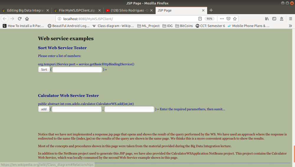
This is the assignment I did for this part of the course, the Netbeans project is available here: File:MyWSJSPClient.zip

The following image is the Web Application created from MyWSJSPClient:

Java Web Application that consume two Web Services. The Sort Web Service Tester is consume from http://vhost3.cs.rit.edu/SortServ/Service.svc?Wsdl. The Calculator Web Service is locally consumed from the CalculatorWSApplication project we created at Big Data Integration#Creating - Deploying and Testing a Java Web Service using NetBeans

Another example 2 - Creating a Java Web Application that consume a Web Service using NetBeans

In this page we can find another example of a Java EE web application that contains a web service: https://netbeans.org/kb/docs/websvc/flower_overview.html

Data analysis

Data analysis is the process of inspecting, cleansing, transforming, and modelling data with a goal of discovering useful information, suggesting conclusions, and supporting decision-making.

Data mining is a particular data analysis technique that focuses on the modelling and knowledge discovery for predictive rather than purely descriptive purposes, while business intelligence covers data analysis that relies heavily on aggregation, focusing on business information.

In statistical applications, data analysis can be divided into:

• Descriptive statistics,
• Exploratory data analysis (EDA), and
• Confirmatory data analysis (CDA).

In particular, data analysis typically includes data retrieval and data cleaning (pre-processing) stages.

Exploratory Data: In statistics, the exploratory data analysis (EDA) is an approach to analyzing data sets to summarize their main characteristics, often with visual methods.

Confirmatory Analysis: In statistics, confirmatory analysis (CA) or confirmatory factor analysis (CFA) is a special form of factor analysis, most commonly used in social research.

Empirical Research:

Statistical Significance:

Descriptive Data Analysis:

• Rather than find hidden information in the data, descriptive data analysis looks to summarise the dataset.
• They are commonly implemented measures included in the descriptive data analysis:
  • Central tendency (mean, mode, median)
  • Variability (standard deviation, min/max)

Exploratory Data Analysis:

• Generate Summaries and make general statements about the data, and its relationships within the data is the heart of Exploratory Data Analysis.

• We generally make assumptions on the entire population but mostly just work with small samples. Why are we allowed to do this??? Two important definitions:
  • Population: A precise definition of all possible outcomes, measurements or values for which inference will be made about.
  • Sample: A portion of the population which is representative of the population (at least ideally).

Types of Variable: https://statistics.laerd.com/statistical-guides/types-of-variable.php

Central tendency

https://statistics.laerd.com/statistical-guides/measures-central-tendency-mean-mode-median.php

A central tendency (or measure of central tendency) is a single value that attempts to describe a set of data by identifying the central position within that set of data.

The mean (often called the average) is most likely the measure of central tendency that you are most familiar with, but there are others, such as the median and the mode.

The mean, median and mode are all valid measures of central tendency, but under different conditions, some measures of central tendency become more appropriate to use than others. In the following sections, we will look at the mean, mode and median, and learn how to calculate them and under what conditions they are most appropriate to be used.

Mean

Mean (Arithmetic)

The mean (or average) is the most popular and well known measure of central tendency.

The mean is equal to the sum of all the values in the data set divided by the number of values in the data set.

So, if we have $n$ values in a data set and they have values $x_{1},x_{2},...,x_{n},$the sample mean, usually denoted by ${\bar {x}}$ (pronounced x bar), is:

${\bar {x}}={\frac {(x_{1}+x_{2}+...+x_{n})}{n}}={\frac {\sum x}{n}}$

The mean is essentially a model of your data set. It is the value that is most common. You will notice, however, that the mean is not often one of the actual values that you have observed in your data set. However, one of its important properties is that it minimises error in the prediction of any one value in your data set. That is, it is the value that produces the lowest amount of error from all other values in the data set.

An important property of the mean is that it includes every value in your data set as part of the calculation. In addition, the mean is the only measure of central tendency where the sum of the deviations of each value from the mean is always zero.

When not to use the mean

The mean has one main disadvantage: it is particularly susceptible to the influence of outliers. These are values that are unusual compared to the rest of the data set by being especially small or large in numerical value. For example, consider the wages of staff at a factory below:

Staff	1	2	3	4	5	6	7	8	9	10
Salary	$15k$	$18k$	$16k$	$14k$	$15k$	$15k$	$12k$	$17k$	$90k$	$95k$

The mean salary for these ten staff is $30.7k. However, inspecting the raw data suggests that this mean value might not be the best way to accurately reflect the typical salary of a worker, as most workers have salaries in the $12k to 18k range. The mean is being skewed by the two large salaries. Therefore, in this situation, we would like to have a better measure of central tendency. As we will find out later, taking the median would be a better measure of central tendency in this situation.

Another time when we usually prefer the median over the mean (or mode) is when our data is skewed (i.e., the frequency distribution for our data is skewed). If we consider the normal distribution - as this is the most frequently assessed in statistics - when the data is perfectly normal, the mean, median and mode are identical. Moreover, they all represent the most typical value in the data set. However, as the data becomes skewed the mean loses its ability to provide the best central location for the data because the skewed data is dragging it away from the typical value. However, the median best retains this position and is not as strongly influenced by the skewed values. This is explained in more detail in the skewed distribution section later in this guide.

Mean in R

mean(iris$Sepal.Width)

Median

The median is the middle score for a set of data that has been arranged in order of magnitude. The median is less affected by outliers and skewed data. In order to calculate the median, suppose we have the data below:

65	55	89	56	35	14	56	55	87	45	92

We first need to rearrange that data into order of magnitude (smallest first):

14	35	45	55	55	56	56	65	87	89	92

Our median mark is the middle mark - in this case, 56. It is the middle mark because there are 5 scores before it and 5 scores after it. This works fine when you have an odd number of scores, but what happens when you have an even number of scores? What if you had only 10 scores? Well, you simply have to take the middle two scores and average the result. So, if we look at the example below:

65	55	89	56	35	14	56	55	87	45

We again rearrange that data into order of magnitude (smallest first):

14	35	45	55	55	56	56	65	87	89

Only now we have to take the 5th and 6th score in our data set and average them to get a median of 55.5.

Median in R

median(iris$Sepal.Length)

Mode

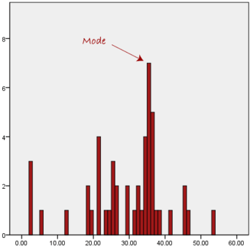
The mode is the most frequent score in our data set. On a histogram it represents the highest bar in a bar chart or histogram. You can, therefore, sometimes consider the mode as being the most popular option. An example of a mode is presented below:

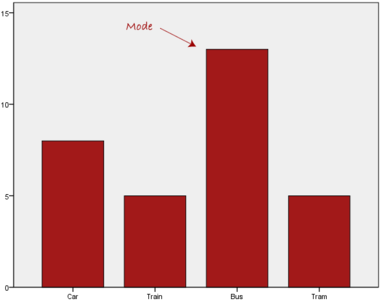
Normally, the mode is used for categorical data where we wish to know which is the most common category, as illustrated below:

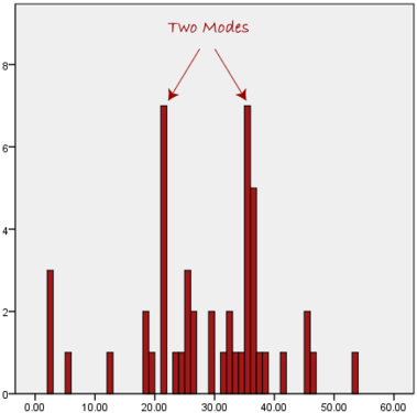
We can see above that the most common form of transport, in this particular data set, is the bus. However, one of the problems with the mode is that it is not unique, so it leaves us with problems when we have two or more values that share the highest frequency, such as below:

We are now stuck as to which mode best describes the central tendency of the data. This is particularly problematic when we have continuous data because we are more likely not to have any one value that is more frequent than the other. For example, consider measuring 30 peoples' weight (to the nearest 0.1 kg). How likely is it that we will find two or more people with exactly the same weight (e.g., 67.4 kg)? The answer, is probably very unlikely - many people might be close, but with such a small sample (30 people) and a large range of possible weights, you are unlikely to find two people with exactly the same weight; that is, to the nearest 0.1 kg. This is why the mode is very rarely used with continuous data.

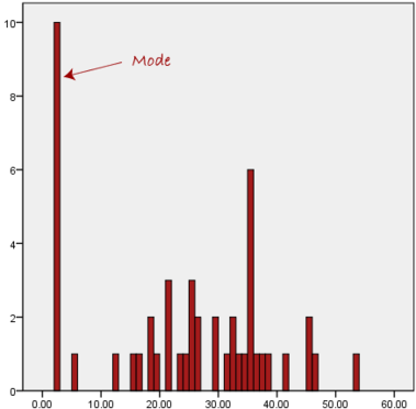
Another problem with the mode is that it will not provide us with a very good measure of central tendency when the most common mark is far away from the rest of the data in the data set, as depicted in the diagram below:

In the above diagram the mode has a value of 2. We can clearly see, however, that the mode is not representative of the data, which is mostly concentrated around the 20 to 30 value range. To use the mode to describe the central tendency of this data set would be misleading.

To get the Mode in R

install.packages("modeest")
library(modeest)

> mfv(iris$Sepal.Width, method = "mfv")

Skewed Distributions and the Mean and Median

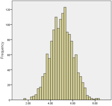
We often test whether our data is normally distributed because this is a common assumption underlying many statistical tests. An example of a normally distributed set of data is presented below:

When you have a normally distributed sample you can legitimately use both the mean or the median as your measure of central tendency. In fact, in any symmetrical distribution the mean, median and mode are equal. However, in this situation, the mean is widely preferred as the best measure of central tendency because it is the measure that includes all the values in the data set for its calculation, and any change in any of the scores will affect the value of the mean. This is not the case with the median or mode.

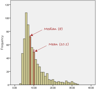
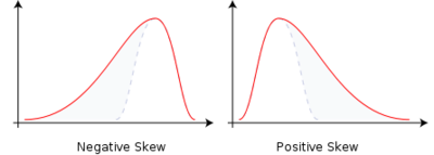
However, when our data is skewed, for example, as with the right-skewed data set below:

we find that the mean is being dragged in the direct of the skew. In these situations, the median is generally considered to be the best representative of the central location of the data. The more skewed the distribution, the greater the difference between the median and mean, and the greater emphasis should be placed on using the median as opposed to the mean. A classic example of the above right-skewed distribution is income (salary), where higher-earners provide a false representation of the typical income if expressed as a mean and not a median.

If dealing with a normal distribution, and tests of normality show that the data is non-normal, it is customary to use the median instead of the mean. However, this is more a rule of thumb than a strict guideline. Sometimes, researchers wish to report the mean of a skewed distribution if the median and mean are not appreciably different (a subjective assessment), and if it allows easier comparisons to previous research to be made.

Summary of when to use the mean, median and mode

Please use the following summary table to know what the best measure of central tendency is with respect to the different types of variable:

Type of Variable	Best measure of central tendency
Nominal	Mode
Ordinal	Median
Interval/Ratio (not skewed)	Mean
Interval/Ratio (skewed)	Median

For answers to frequently asked questions about measures of central tendency, please go to: https://statistics.laerd.com/statistical-guides/measures-central-tendency-mean-mode-median-faqs.php

Measures of Variation

Range

The Range just simply shows the min and max value of a variable.

In R:

> min(iris$Sepal.Width)
> max(iris$Sepal.Width)
> range(iris$Sepal.Width)

Range can be used on Ordinal, Ratio and Interval scales

Quartile

https://statistics.laerd.com/statistical-guides/measures-of-spread-range-quartiles.php

Quartiles tell us about the spread of a data set by breaking the data set into quarters, just like the median breaks it in half.

For example, consider the marks of the 100 students, which have been ordered from the lowest to the highest scores.

• The first quartile (Q1): Lies between the 25th and 26th student's marks.
  • So, if the 25th and 26th student's marks are 45 and 45, respectively:
    • (Q1) = (45 + 45) ÷ 2 = 45
• The second quartile (Q2): Lies between the 50th and 51st student's marks.
  • If the 50th and 51th student's marks are 58 and 59, respectively:
    • (Q2) = (58 + 59) ÷ 2 = 58.5
• The third quartile (Q3): Lies between the 75th and 76th student's marks.
  • If the 75th and 76th student's marks are 71 and 71, respectively:
    • (Q3) = (71 + 71) ÷ 2 = 71

In the above example, we have an even number of scores (100 students, rather than an odd number, such as 99 students). This means that when we calculate the quartiles, we take the sum of the two scores around each quartile and then half them (hence Q1= (45 + 45) ÷ 2 = 45) . However, if we had an odd number of scores (say, 99 students), we would only need to take one score for each quartile (that is, the 25th, 50th and 75th scores). You should recognize that the second quartile is also the median.

Quartiles are a useful measure of spread because they are much less affected by outliers or a skewed data set than the equivalent measures of mean and standard deviation. For this reason, quartiles are often reported along with the median as the best choice of measure of spread and central tendency, respectively, when dealing with skewed and/or data with outliers. A common way of expressing quartiles is as an interquartile range. The interquartile range describes the difference between the third quartile (Q3) and the first quartile (Q1), telling us about the range of the middle half of the scores in the distribution. Hence, for our 100 students:

$Interquartile\ range=Q3-Q1=71-45=26$

However, it should be noted that in journals and other publications you will usually see the interquartile range reported as 45 to 71, rather than the calculated $Interquartile\ range.$

A slight variation on this is the $semi{\text{-}}interquartilerange,$which is half the $Interquartile\ range.$Hence, for our 100 students:

$Semi{\text{-}}Interquartile\ range={\frac {Q3-Q1}{2}}={\frac {71-45}{2}}=13$

Quartile in R

quantile(iris$Sepal.Length)

Result 
0%    25%    50%    75%    100% 
4.3   5.1    5.8    6.4    7.9

0% and 100% are equivalent to min max values.

Box Plots

boxplot(iris$Sepal.Length,
       col = "blue", 
       main="iris dataset", 
       ylab = "Sepal Length")

Variance

https://statistics.laerd.com/statistical-guides/measures-of-spread-absolute-deviation-variance.php

Another method for calculating the deviation of a group of scores from the mean, such as the 100 students we used earlier, is to use the variance. Unlike the absolute deviation, which uses the absolute value of the deviation in order to "rid itself" of the negative values, the variance achieves positive values by squaring each of the deviations instead. Adding up these squared deviations gives us the sum of squares, which we can then divide by the total number of scores in our group of data (in other words, 100 because there are 100 students) to find the variance (see below). Therefore, for our 100 students, the variance is 211.89, as shown below:

$variance=\sigma ={\frac {\sum (X-\mu )^{2}}{N}}$

$\mu :{\text{Mean}};\ \ \ X:{\text{Score}};\ \ \ N:{\text{Number of scores}}$

• Variance describes the spread of the data.
• It is a measure of deviation of a variable from the arithmetic mean.
• The technical definition is the average of the squared differences from the mean.
• A value of zero means that there is no variability; All the numbers in the data set are the same.
• A higher number would indicate a large variety of numbers.
  

Variance in R

var(iris$Sepal.Length)

Standard Deviation

https://statistics.laerd.com/statistical-guides/measures-of-spread-standard-deviation.php

The standard deviation is a measure of the spread of scores within a set of data. Usually, we are interested in the standard deviation of a population. However, as we are often presented with data from a sample only, we can estimate the population standard deviation from a sample standard deviation. These two standard deviations - sample and population standard deviations - are calculated differently. In statistics, we are usually presented with having to calculate sample standard deviations, and so this is what this article will focus on, although the formula for a population standard deviation will also be shown.

The sample standard deviation formula is:

$s={\sqrt {\frac {\sum (X-{\bar {X}})^{2}}{n-1}}}$

${\bar {X}}:{\text{Sample mean}};\ \ \ n:{\text{Number of scores in the sample}}$

The population standard deviation formula is:

$\sigma ={\sqrt {\frac {\sum (X-\mu )^{2}}{n}}}$

$\mu :{\text{population mean}}$

• The Standard Deviation is the square root of the variance.
• This measure is the most widely used to express deviation from the mean in a variable.
• The higher the value the more widely distributed are the variable data values around the mean.
• Assuming the frequency distributions approximately normal, about 68% of all observations are within +/- 1 standard deviation.
• Approximately 95% of all observations fall within two standard deviations of the mean (if data is normally distributed).

Standard Deviation in R

sd(iris$Sepal.Length)

Z Score

• z-score represents how far from the mean a particular value is based on the number of standard deviations.
• z-scores are also known as standardized residuals
• Note: mean and standard deviation are sensitive to outliers

> x <-((iris$Sepal.Width) - mean(iris$Sepal.Width))/sd(iris$Sepal.Width)
> x 
> x[77] #choose a single row # or this
> x <-((iris$Sepal.Width[77]) - mean(iris$Sepal.Width))/sd(iris$Sepal.Width)
> x

Shape of Distribution

Skewness

• Skewness is a method for quantifying the lack of symmetry in the distribution of a variable.

• Skewness value of zero indicates that the variable is distributed symmetrically. Positive number indicate asymmetry to the left, negative number indicates asymmetry to the right.

Skewness in R

> install.packages("moments") and library(moments)
> skewness(iris$Sepal.Width)

Histograms in R

> hist(iris$Petal.Width)

Kurtosis

• Kurtosis is a measure that gives indication in terms of the peak of the distribution.

• Variables with a pronounced peak toward the mean have a high Kurtosis score and variables with a flat peak have a low Kurtosis score.

Kurtosis in R

> kurtosis(iris$Sepal.Length)

Correlations

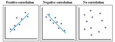
Correlation give us a measure of the relation between two or more variables.

• Positive correlation: The points lie close to a straight line, which has a positive gradient. This shows that as one variable increases the other increases.

• Negative correlation: The points lie close to a straight line, which has a negative gradient. This shows that as one variable increases the other decreases.

• No correlation: There is no pattern to the points. This shows that there is no correlation between the tow variables.

Simple Linear Correlation

• Looking for the extent to which two values of the two variables are proportional to each other.

• Summarised by a straight line.

• This line is called a Regression Line or a Least Squares Line.

• It is determined by maintaining the lowest possible sum of squared distances between the data points and the line.

• We must use interval scales or ratio scales for this type of analysis.

Simple Linear Correlation in R

Example 1:

> install.packages('ggplot2')
> library(ggplot2)
> data("iris")

> ggplot(iris, aes(x=Sepal.Length, y=Sepal.Width)) + 
         geom_point(color='black') + 
         geom_smooth(method=lm, se=FALSE, fullrange=TRUE)

Example 2:

> library(ggplot2)
> data("iris")
> ggplot(iris, aes(x=Petal.Length, y=Sepal.Length)) + 
         geom_point(color='black') + 
         geom_smooth(method=lm, se=FALSE, fullrange=TRUE)

Apache Hadoop

https://hadoop.apache.org/docs/r2.7.7/

Hadoop is an open-source software framework for storing data and running applications on clusters of commodity hardware. It provides massive storage for any kind of data, enormous processing power and the ability to handle virtually limitless concurrent tasks or jobs. https://www.sas.com/en_ie/insights/big-data/hadoop.html

Apache Hadoop is a collection of open-source software utilities that facilitate using a network of many computers to solve problems involving massive amounts of data and computation. It provides a software framework for distributed storage and processing of big data using the MapReduce programming model. https://en.wikipedia.org/wiki/Apache_Hadoop

Single Node Setup

https://hadoop.apache.org/docs/r1.2.1/single_node_setup.html

This document describes how to set up and configure a single-node Hadoop installation so that you can quickly perform simple operations using Hadoop MapReduce and the Hadoop Distributed File System (HDFS).

MapReduce

https://hadoop.apache.org/docs/r1.2.1/mapred_tutorial.html

Hadoop MapReduce is a software framework for easily writing applications which process vast amounts of data (multi-terabyte data-sets) in-parallel on large clusters (thousands of nodes) of commodity hardware in a reliable, fault-tolerant manner.

A MapReduce job usually splits the input data-set into independent chunks which are processed by the map tasks in a completely parallel manner. The framework sorts the outputs of the maps, which are then input to the reduce tasks. Typically both the input and the output of the job are stored in a file-system. The framework takes care of scheduling tasks, monitoring them and re-executes the failed tasks.

Inputs and Outputs0

The MapReduce framework operates exclusively on <key, value> pairs, that is, the framework views the input to the job as a set of <key, value> pairs and produces a set of <key, value> pairs as the output of the job, conceivably of different types.

The key and value classes have to be serializable by the framework and hence need to implement the Writable interface. Additionally, the key classes have to implement the WritableComparable interface to facilitate sorting by the framework.

Input and Output types of a MapReduce job:

(input) <k1, v1> -> map -> <k2, v2> -> combine -> <k2, v2> -> reduce -> <k3, v3> (output)

Example - WordCount

Before we jump into the details, lets walk through an example MapReduce application to get a flavour for how they work.

WordCount is a simple application that counts the number of occurences of each word in a given input set.

This works with a local-standalone, pseudo-distributed or fully-distributed Hadoop installation (Single Node Setup).

Hadoop Architecture

• Distributed, with some centralization.

• Main nodes of cluster are where most of the computational power and storage of the system lies.

• Main nodes run TaskTracker to accept and reply to MapReduce tasks, and also DataNode to store needed blocks closely as possible.

• Central control node runs NameNode to keep track of HDFS directories & files, and JobTracker to dispatch compute tasks to TaskTracker.

• Written in Java, also supports Python and Ruby.

Hadoop framework includes following four modules:

• Hadoop Common: These are Java libraries and utilities required by other Hadoop modules. These libraries provide the file system and OS level abstractions and contain the necessary Java files and scripts required to start Hadoop.
• Hadoop Distributed File System (HDFS): A distributed file system that provides high-throughput access to the application data.
• Hadoop YARN: This is a framework for the job scheduling and cluster resource management.
• Hadoop MapReduce: This is a YARN-based system for parallel processing of large data sets.

Hadoop Operation Modes:

• Local/ Standalone Mode: After downloading Hadoop in your system, by default, it is configured in a standalone mode and can be run as a single java process.
• Pseudo Distributed Mode: It is a distributed simulation on a single machine. Each Hadoop daemon such as hdfs, yarn, MapReduce etc., will run as a separate java process. This mode is useful for development.
• Fully Distributed Mode: This mode is fully distributed with minimum two or more machines as a cluster. This is what you would get from AWS.

Hadoop Framework Tools:

• Hbase: HBase is an open-source, non-relational, distributed database modelled after Google's Bigtable and written in Java.

• Chukwa: Chukwa is a Hadoop subproject devoted to large-scale log collection and analysis. Chukwa is built on top of the Hadoop distributed filesystem (HDFS) and MapReduce framework and inherits Hadoop’s scalability and robustness.

• Flume: Flume is a distributed, reliable, and available service for efficiently collecting, aggregating, and moving large amounts of log data. It has a simple and flexible architecture based on streaming data flows.

• Apache ZooKeeper: Apache ZooKeeper is a centralized service for maintaining configuration information, naming, providing distributed synchronization, and providing group services.

• Apache Pig: Apache Pig is a platform for analyzing large data sets that consists of a high-level language for expressing data analysis programs, coupled with infrastructure for evaluating these programs.

• Apache Hive: Apache Hive is a data warehouse software project built on top of Apache Hadoop for providing data query and analysis. Hive gives a SQL-like interface to query data stored in various databases and file systems that integrate with Hadoop.

• Apache Sqoop(TM) is a tool designed for efficiently transferring bulk data between Apache Hadoop and structured datastores such as relational databases.

• Apache Avro is a remote procedure call and data serialization framework developed within Apache's Hadoop project. It uses JSON for defining data types and protocols, and serializes data in a compact binary format.

HDFS

• HDFS is a file system written in Java based on the Google’s file system (GFS).
• Provides the redundant storage for massive amounts of data.
• All HDFS communication protocols are layered on top of the TCP/IP protocol.
• A client establishes a connection to a configurable TCP port on the Namenode machine. It talks to ClientProtocol with the Namenode.
• Namenode keeps the directory tree of all files in the file system, and tracks where across the cluster the file data is kept.

• Chunking:

• When you upload a file to HDFS, the file is first chunked into blocks of a fixed size, typically between 64MB and 256MB.

• Replication & Distribution:

• Each block is replicated across multiple datanodes (typically 3) that are chosen at random.
• A DataNode stores data in the [HadoopFileSystem]. A functional filesystem has more than one DataNode, with data replicated across them.

• Features of HDFS:

• It is suitable for the distributed storage and processing.

• Hadoop provides a command line interface to interact with HDFS.

• The built-in servers of namenode and datanode help users to easily check the status of a cluster.

• Streaming access to file system data.

• HDFS provides file permissions and authentication.

• HDFS Commands:

• The syntax of the commands is similar to bash.

• Make a directory:

$ hadoop fs -mkdir  user

• List contents of directory

$ hadoop fs -ls user

• List contents of a sub directory

$ hadoop fs -ls user/subDir

• Files Stored :

• Files are divided into blocks.
• Blocks are divided across many machines at load time.
• Different blocks from the same file will be stored on different machines.
• Blocks are replicated across multiple machines.
• The NameNode keeps track of which blocks make up a file and where they are stored.

• Namenode:

• The system having the namenode acts as the master server and it does the following tasks:

• Manages the file system namespace.
• Regulates client’s access to files.
• It also executes file system operations, such as renaming, closing, and opening files and directories.

• Datanode:

• For every node (Commodity hardware/ System) in a cluster, there will be a datanode. These nodes manage the data storage of their system.
• Datanodes perform read-write operations on the file systems, as per client request.
• They also perform operations, such as block creation, deletion, and replication according to the instructions of the namenode.

MapReduce

• MapReduce is a processing technique and a program model for distributed computing based on java.
• The MapReduce algorithm contains two important tasks, namely Map and Reduce.
• Map takes a set of data and converts it into another set of data, where individual elements are broken down into tuples (key/value pairs).
• Secondly, reduce task, which takes the output from a map as an input and combines those data tuples into a smaller set of tuples.

• As the sequence of the name MapReduce implies, the reduce task is always performed after the map job.
• The major advantage of MapReduce is that it is easy to scale data processing over multiple computing nodes.
• Scaling the application to run over hundreds, thousands, or even tens of thousands of machines in a cluster is merely a configuration change.
• This simple scalability is what has attracted many programmers to use the MapReduce model.

• Map Stage: The map or mapper’s job is to process the input data. Generally the input data is in the form of file or directory and is stored in the Hadoop file system (HDFS). The input file is passed to the mapper function line by line. The mapper processes the data and creates several small chunks of data.

• Reduce Stage: This stage is the combination of the Shuffle stage and the Reduce stage. The Reducer’s job is to process the data that comes from the mapper. After processing, it produces a new set of output, which will be stored in the HDFS.

• MapReduce Steps:

• Splitting – The splitting parameter can be anything, e.g. splitting by space, comma, semicolon, or even by a new line (‘\n’).
• Mapping – It takes a set of data and converts it into another set of data, where individual elements are broken down into tuples (Key-Value pair).
• Intermediate splitting – The entire process is performed in parallel on different clusters. In order to group them in “Reduce Phase” the similar KEY data should be on same cluster.
• Reduce – It is mostly a group by phase.
• Combining – The last phase where all the data (individual result set from each cluster) is combined together to form a Result.

• Example map (I):

function map(values, f) {
  var results = [];
  for (var i = 0 ; i < values.length ; i++) {
    results.push(f(values[i]));
  }
  return results;
}

• Here's a Javascript implementation of map

• Create a new array
• Apply the function f to each element of the input array (values) and append (push in Javascript) the result to the output array

Three main applications of Hadoop

• Advertisement (Mining user behavior to generate recommendations)

• Searches (group related documents)

• Security (search for uncommon patterns)

Rails

https://guides.rubyonrails.org/getting_started.html

https://en.wikipedia.org/wiki/Ruby_on_Rails

Ruby on Rails, or Rails, is a server-side web application framework written in Ruby under the MIT License. Rails is a model-view-controller (MVC) framework, providing default structures for a database, a web service, and web pages. It encourages and facilitates the use of web standards such as JSON or XML for data transfer, HTML, CSS and JavaScript for user interfacing.

Installation

Ruby installation:

sudo apt install ruby

Rails installation:

sudo apt install ruby-railties
sudo apt-get install rails

For gem installation:

sudo apt-get install gem
sudo apt-get install nodejs
sudo gem install bundler

How to create a Rails Application

When you install the Rails framework, you also get a new command-line tool, rails, that is used to construct each new Rails application you write.

Why do we need a tool? Why can't we just hack away in our favorite editor and create the source for our application from scratch? Well, we could just hack; after all, a Rails application is just Ruby source code. But Rails also does a lot of magic behind the curtain to get our application to work with a minumum of explicit configuration. To get this magic to work, Rails needs to find all the various componenets of your application. Aas we'll see later, this means we need to create a specific directory structure, slotting the code we write into the appropriate places. The rails command simply creates this directory structure for us and populates it with some standards Rails code.

To create your first Rails application:

rails new myrailsapp

The above command has created a directory named myrailsapp.

Examine your installation using the following command:

rake about

Once you get rake about working, you have everything you need to start a standar-alone web server that can run our newly created Rails application. So, let's star our demos application:

rails server

Rails 4.2.10 application starting in development on http://localhost:3000

At this point, we have a new application running, but it has none of our code in it.

Hello Rails

Let's start by creating a "Hello, world!"

Rails is a Model-View-Controller framework. Rails accepts incoming request from a browser, decodes the request to find a controller, and calls an action method in that controller. The controller then invokes a particular view to display the results to the user. To write our simple "Hello World!" application, we need code for a controller and a view, and we need a route to connect the two. We don't need code for a model, because we're not dealing with any data. Let's start with the controller.

In the same way that we used the rails commands to create a new Rails application, we can also use a generator script to create a new controller for our project. This command is called rails generate . So, to create a controller called say, we run the command passing in the name of the controller we want to create and the names of the actions we intend for this controller to support:

rails generate controller Say hello goodbye

      create  app/controllers/say_controller.rb
       route  get 'say/goodbye'
       route  get 'say/hello'
      invoke  erb
      create    app/views/say
      create    app/views/say/hello.html.erb
      create    app/views/say/goodbye.html.erb
      invoke  test_unit
      create    test/controllers/say_controller_test.rb
      invoke  helper
      create    app/helpers/say_helper.rb
      invoke    test_unit
      invoke  assets
      invoke    coffee
      create      app/assets/javascripts/say.coffee
      invoke    scss
      create      app/assets/stylesheets/say.scss

Notice the files that were generated for the rails generate command. The first source file we'll be looking at is the controller:

app/controllers/say_controller.rb

class SayController < ApplicationController
  def hello
  end

  def goodbye
  end
end

SayController is a class that inherits from ApplicationController, so it automatically gets all the default controller behavior. What does this code have to do? For now, it does nothing, we sinply have empty action methods named hello() and goodbye(). To understand why these methods are named this way, we need to look at the way Rails handles requests.

Rails and Request URLs

Like any other web application, a Rails application appears to its users to be associated with a URL. When you point your browser at that URL, you are talking to the application code, which generates a respondse to you.

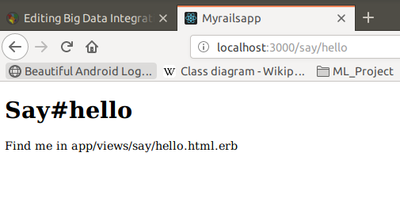
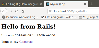
Let's try it now. Navigate to the URL http://localhost:3000/say/hello

You'll see something that looks like this:

Our first action

At this point, we can see not only that we have connected the URL to our controller but also tat Rails is pointing the way to our next step, namely, to tell Rails what to display. That's where views come in. Remember when we ran the script to create the new controller? That command added several files and a new directory to our application. That directory contains the template files to the controller's view. In our case, we created a controller named say, so the view will be in the directory app/views/say.

By default, Rails looks for templates in a file with the same name as the action it's handling. In our case, that means we need to replace a file called hello.html.erb in the directory app/views/say. (Why .html.erb? We'll explain in a minute.) For now, let's just put some basic HTML in there:

app/views/say/hello.html.erb

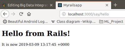
<h1>Hello from Rails!</h1>

Save the file hello.html.erb and refresh your browser.

In total, we've looked at two files in our Rails application tree. We looked at the controller, and we modified a template to display a page in the browser.

These files live in standard locations in the Rails hierarchy: controllers go into app/controllers, and views go into sub-directories of app/views:

.
├── app
│   ├── assets
│   │   ├── images
│   │   ├── javascripts
│   │   │   ├── application.js
│   │   │   └── say.coffee
│   │   └── stylesheets
│   │       ├── application.css
│   │       └── say.scss
│   ├── controllers
│   │   ├── application_controller.rb
│   │   ├── concerns
│   │   └── 'say_controller.rb'
│   ├── helpers
│   │   ├── application_helper.rb
│   │   └── say_helper.rb
│   ├── mailers
│   ├── models
│   │   └── concerns
│   └── views
│       ├── layouts
│       │   └── application.html.erb
│       └── say
│           ├── goodbye.html.erb
│           └── 'hello.html.erb'
├── bin
│   ├── bundle
│   ├── rails
│   ├── rake
    .
    .
    .

Making it dynamic

So far, our Rails application is pretty boring, it just displays a static page. To make it more dynamic, let's have it show the current time each time it displays the page.

To do this, we need to change the template file in the view, it now needs to include the time as a string. That raises two questions. First, how do we add dynamic content to a template? Second, where do we get the time from?

Dynamic content

There are many ways of creating dynamic templates in Rails. The most common way, which we'll use here, is to embed Ruby code in the template. That's why we nemed our template file hello.html.erb; the '.html.erb suffix tells Rails to expand the content in the file using a system called ERB.

ERB is a filter that is installed as part of the Rails installation that takes an .erbfile and outputs a tranformed version. The output file is often HTML in Rails, but it can be anyting. Normal content is passed through without being changed. However, content between <%= and %> is interpreted as Ruby code and executed. The result of that exwcution is converted into a string, and that value is subtituted in the file in place of the <%=...%> sequence. For example, chage hello.html.erb to display the current time:

app/views/say/hello.html.erb

<h1>Hello from Rails!</h1>
<p>
    It is now <%= Time.now %>
</p>

Notice that if you hit Refresh in your browse, the time updates each time the page is displayed.

Adding the time

Our original problem was to display the time to users of our application. We now know how to make our application display dynamic data.

The second issue we have to address is working out where to get the time from.

We've shown that the approach of embedding a call to Ruby's Time.now() method in our hello.html.erb template works. Each time we access this page, the user will see the current time substituted into the body of the response. And for our trivial application, that might be good enough. In general, though, we probably want to do something slightly different. We'll move the determination of the time to be displayed into the controller and leave the view with the simple job of displaying it. We'll change our action method in the controller to set the time value into an instance variable called @time.

app/controllers/say_controller.rb

class SayController < ApplicationController
  def hello
    @time = Time.now
  end

  def goodbye
  end
end

In the .html.erb template, we'll use this instance variable to substitute the time into the output:

app/views/say/hello.html.erb

<h1>Hello from Rails!</h1>
<p>
    It is now <%= @time %>
</p>

When we refresh our browser, we eill again see the current time, showing that the communication between the controller and the view was succesfull.

Why did we go to the extra trouble of setting the time to be displayed in the controller and then using it in the view? Good question. In this application it donen't make much difference, but by putting the logic in the controller instead, we buy ourselves some benefits. For example, we may want to extend our application in the future to support users in many countries. In tat case, we'd want to localize the display of the time, choosing a tie appropriate to their time zone. That would be a fair amount of application-level code, and it would probably not be appropriate to embed it at the view level. By setting the time to display in the controller, we make our application more flexible, we can change the time zone in the controller without having to update any view that uses the time object. The time is data, and is should be supplied to the view by controller. We'll see a lot more of this whewn we introduce models into the equation.

Linking pages together

Normally, each page in your application will correspond to a separate view. In our case, well also use a new action method to handle the page (although that isn't always the case, as we'll see later in the book). We'll use the same controller for both actions. Again, this needn't be the case, but we have no compelling reason to use a new controller right now.

We already defined a goodbye action for this controller, so all that remains is to create a new template in the directory app/views/say. This time it's called goodbye.html.erb because by default templates are named after their associated actions:

app/views/say/goodbye.html.erb

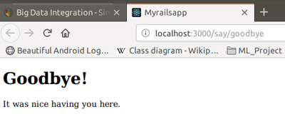
<h1>Goodbye!</h1>
<p>
    It was nice having you here.
</p>

http://localhost:3000/say/goodbye

Now we need to link the two screens. We'll put a link on the hello screen that takes us to the goodbye screen, and vice versa. In a real application, we might want to make these proper buttons, but for now we'll just use hyperlinks.

We already know that Rails uses a convention to parse the URL into a target controller and ac action within that controller. So, a simple approach would be to adopt this URL convention for our links:

app/views/say/hello.html.erb

<h1>Hello from Rails!</h1>
<p>
    It is now <%= @time %>
</p>
<p>
    Say <a href="/say/goodbye">Goodbye</a>!
</p>

and the file goodbye.html.erb would point the other way:

app/views/say/goodbye.html.erb

<h1>Goodbye!</h1>
<p>
    It was nice having you here.
</p>
<p>
    Say <a href="/say/hello">Hello</a>!
</p>

This approach would certainly work, but it's a bit fragile. If we were to move our application to a different place on the web server, the URLs would no longer be valid. It also encodes assumptions about the Rails URL format into our code; it's possible a future version of Rails might change this.

Fortunately, these aren't risks we have to take. Rails comes with a bunch of helper methods that can be used in view templates. Here, we'll use the helper method link_to(), which creates a hyperlink to an action. (The link_to() method can do a lot more that this, but let's take it gently for now) Using link_to(), hello.html.erb becomes the following:

app/views/say/hello.html.erb

<h1>Hello from Rails!</h1>
<p>
    It is now <%= @time %>
</p>
<p>
    Time to say
    <%= link_to "Goodbye", say_goodbye_path %>!
</p>

There's a link_to() call within an ERB <%=...%> sequence. This creates a link to a URL that will invoke the goodbye() action.

We generated the link this way:

link_to "Goodbye", say_goodbye_path

If you come from a language such as Java, you might be surprised that Ruby doesn't insist on parentheses around method parameters. You can always add them if you like.

say_gooodbye_path is a precomputed value that Rails makes available to application views. It evaluates to the /say/goodbye path. Over time you will see that Rails provides the ability to name all the routes that you will be using in your application.

We can make the corresponding chage in goodbye.html.erb:

app/views/say/goodbye.html.erb

<h1>Goodbye!</h1>
<p>
    It was nice having you here.
</p>
<p>
    Say <%= link_to "Hello", say_hello_path %>! again.
</p>

Playtime

Here's some stuff to try on your own:

• Experiment with the follosing expressions:
  • Addition: <%= 1+2 %>
  • Concatenation: <%= "cow" + "boy" %>
  • Time in one hour: <%= 1.hour.from_now.localtime %>

• A call to the followingg Ruby method returns a list of all the files in the current directory:

@files = Dir.glob('*')

use it to set an instance variable in a controller action, and then write the corresponding template that displays the filename in a list on the browser.

Hint: you can iterate over a collection using something like this:

<% for file in @files %>
  file name is: <%= file %>
<% end %>

You might want to use <ul> for the list.

You'll find hints at http://www.pragprog.com/wikis/wiki/RailsPlayTime

The story so far - What we just did

We constructed a toy application that showed us the following:

• How to create a enw Rails application and how to create a new controller in that application.

• How to create dynamic content in the controller and display it via the view template.

• How to link pages together.

Let's briefly review how our current application works:

• The user navigates to our application. In our case, we do that using a local URL such as http://localhost:3000/say/hello

• Rails then matches the route pattern, which it previously split into two parts and analyzed.

The say part is taken to be the name of a controller, so Rails creates a new instance of the Ruby class SayController' (which it finds in app/controllers/say_controller.rb).

• The next part of the pattern, hello', identifies an action. Rails invokes a method of that name in the controller. This action method creates a new time object holding the current time and tucks it away in the @time instance variable.

• Rails looks for a template to display the result. It searches the directory app/views for a subdirectory with the same name as the controller (say) and in that subdirectory for a file named after the action (hello.html.erb).

• Rails processes this file through the ERB templating system, executing and embedded Ruby and substituting in values set up by the controller.

• The result is returned to the browser, and Rails finches processing this request.